r-chitturi

Fun with Filters and Frequencies

Part 1 - Fun with Filters

Part 1.1: Finite Difference Operator

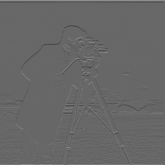
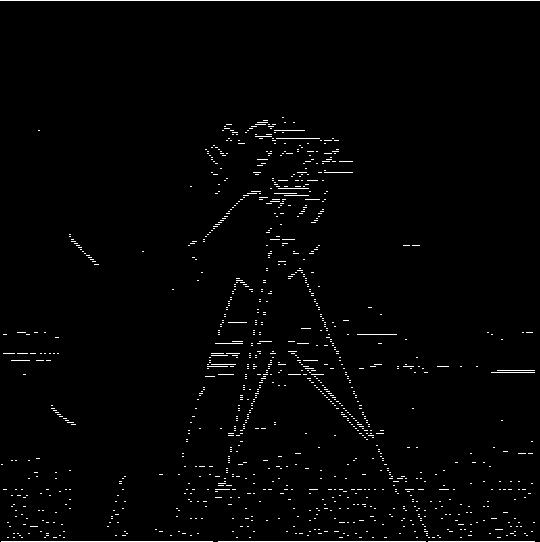
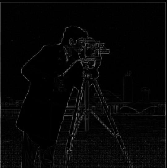
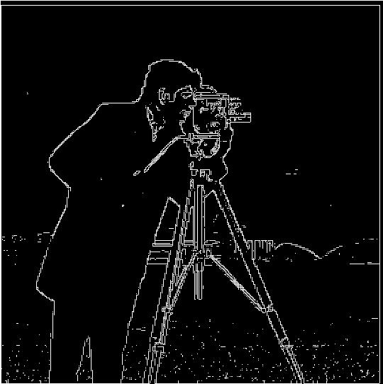
I used the following finite difference operators: dx = np.array([[1, -1]]) and dy = np.array([[1], [-1]]). I convolved these with the cameraman input image by using scipy.signal.convolve2d with mode='same'. I combined the partial derivatives by squaring each, adding them together, and then taking the square root. The threshold for my binary image was 35.

	dx	dy
Derivative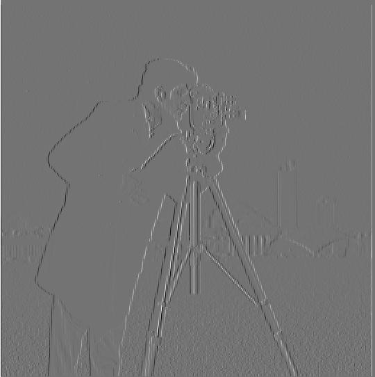
Binarized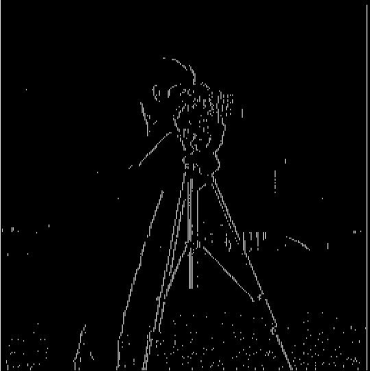

Combined Gradient	Combined Binarized

Part 1.2: Derivative of Gaussian (DoG) Filter

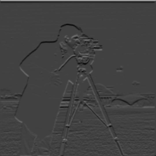
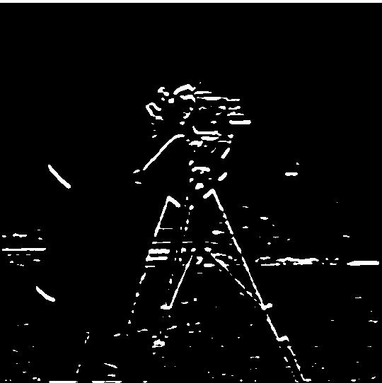
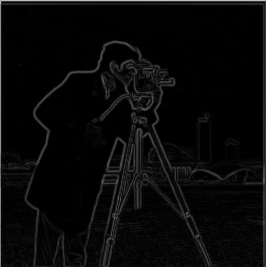
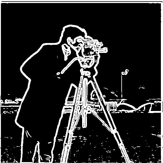
I used the Gaussian kernels to blur the images before using the finite difference operator to generate the partial derivatives. Here, kernel_size = 10 and sigma = kernel_size / 6 Then, we combine them into a single edge image using the same idea from 1.1.

	dx	dy
Derivative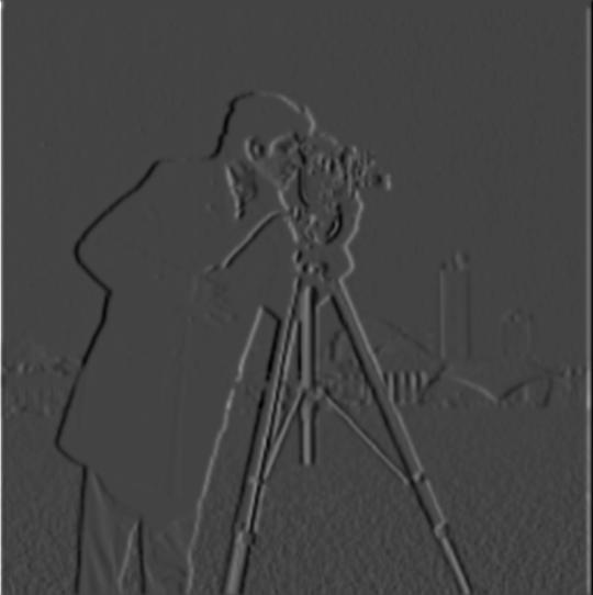
Binarized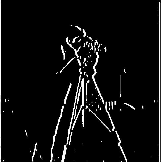

Combined Gradient	Combined Binarized

Comparing Finite Difference and DoG

The results are similar except for small variations in length and shape of smaller edges due to noise. The main difference is that the edges of the DoG filter are thicker and also a bit smoother. Since the Gaussian filter is a low-pass filter, this makes sense since less high frequency components mean less noise and better edge detection.

Binarized Finite Difference	Binarized Derivative of Gaussian

Part 2 - Fun with Frequencies

Part 2.1: Image “Sharpening”

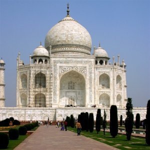
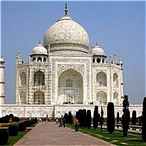
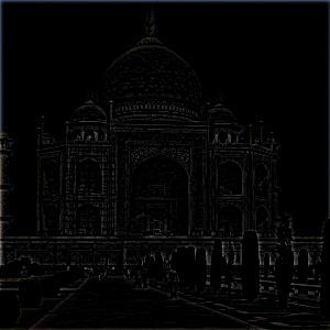
To sharpen an image, we convolve the input image with a gaussian kernel. This acts as a low-pass filter, allowing us to get rid of the higher frequencies. To get the high-frequency details, we use the following operation: details = target_im - blurred_im. This removes the lower frequencies from the original image. We then choose some alpha in order to create the final sharpened image using sharpened_result = target + alpha*details. In the following results, alpha = 1.

Original Image	Sharpened Image	Details

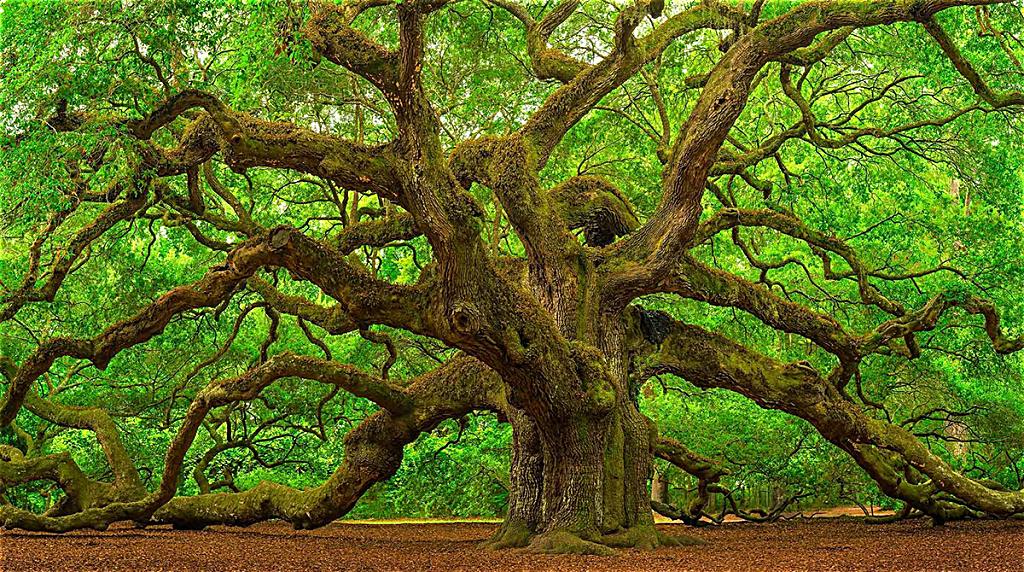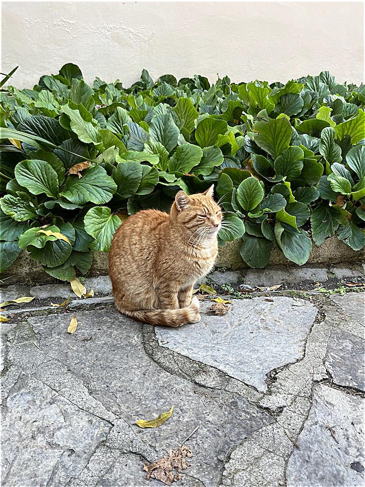
Next, we blur the image of this orange cat using kernel_size = 10 and sigma = kernel_size / 6. We sharpen the image normally with alpha = 1, and then we sharpen the image after blurring with alpha = 2.

Original Image	Sharpened Image	Blurred Image	Blurred then Sharpened

Part 2.2: Hybrid Images

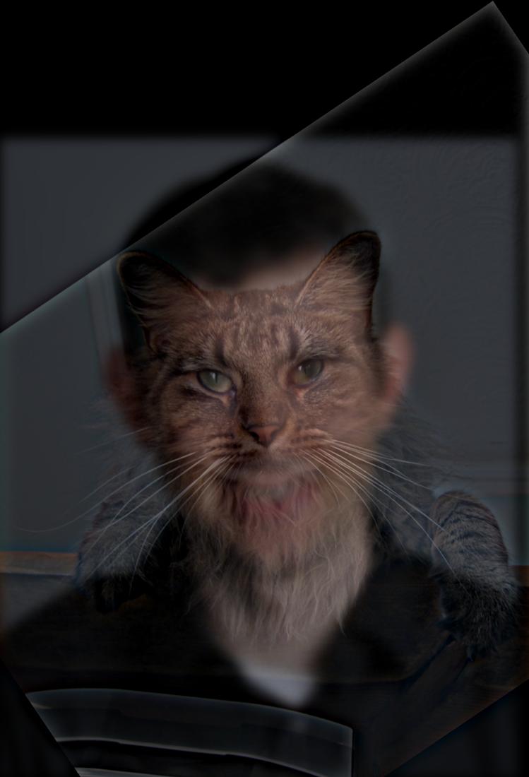
We take in two input images, im_high and im_low, and align them using the provided function. We use a gaussian blur on the high frequency image using kernel_size = 6 * sigma_high to generate blurred_im_high. Then, we get the high frequency image using high = im_high - blurred_im_high. After that, we blur the low frequency image using kernel_size = 6 * sigma_low to get blurred_im_low. We average the pixels of high and blurred_im_low to get our hybrid image!

Low Frequency Image	High Frequency Image	Hybrid Image
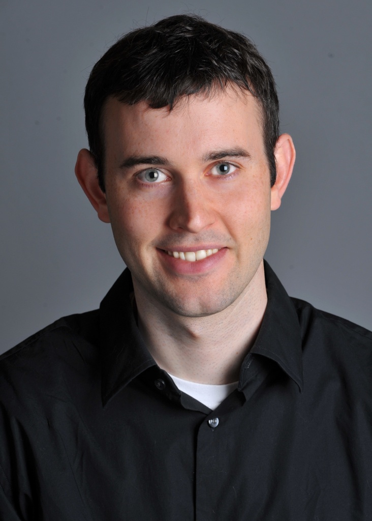Derek	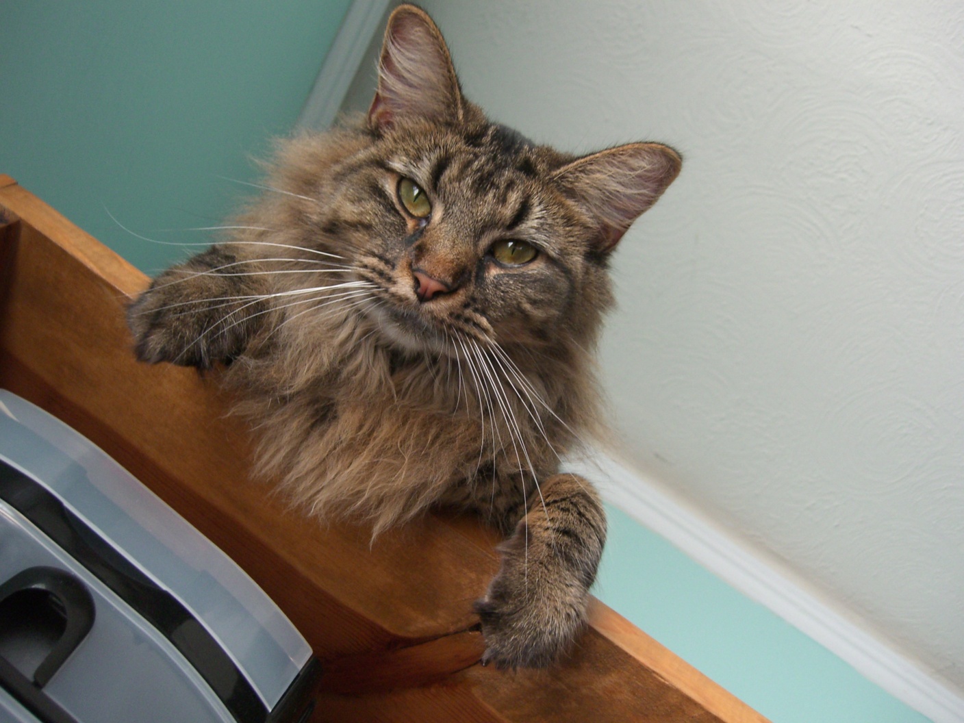Nutmeg	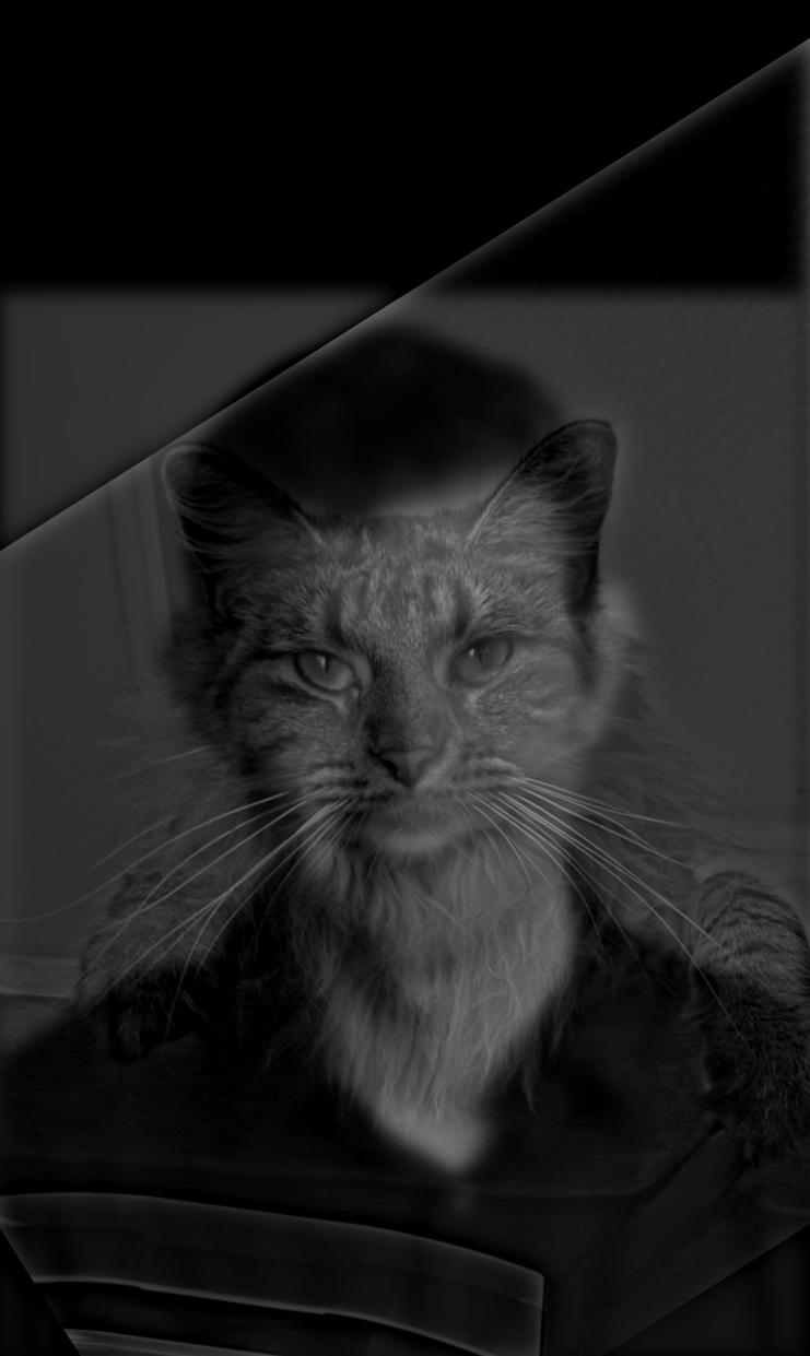sigma_low = 8 sigma_high = 11
Basketball	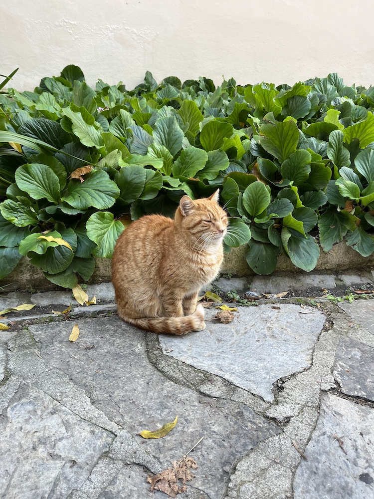Orange Cat	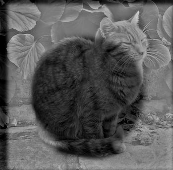sigma_low = 4 sigma_high = 10
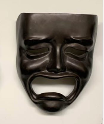Tragedy	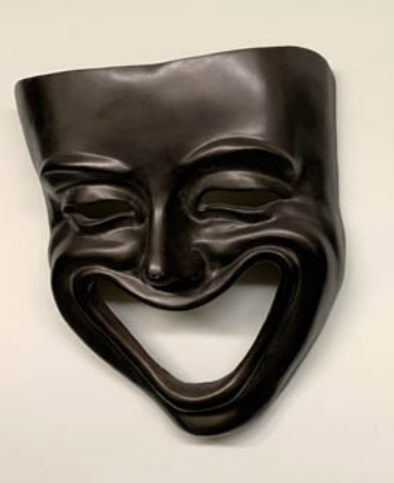Comedy	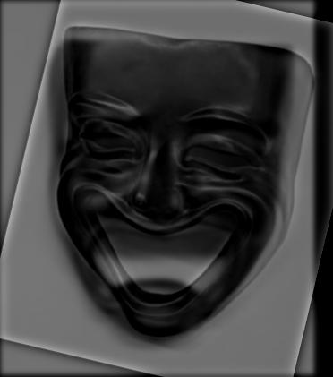sigma_low = 3 sigma_high = 6

The following hybrid image failed, likely because of the paper plane’s thick black lines compared to the airplane.

Low Frequency Image	High Frequency Image	Hybrid Image
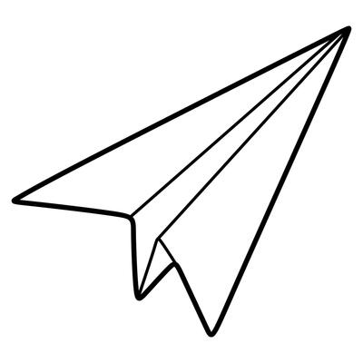Paper Plane	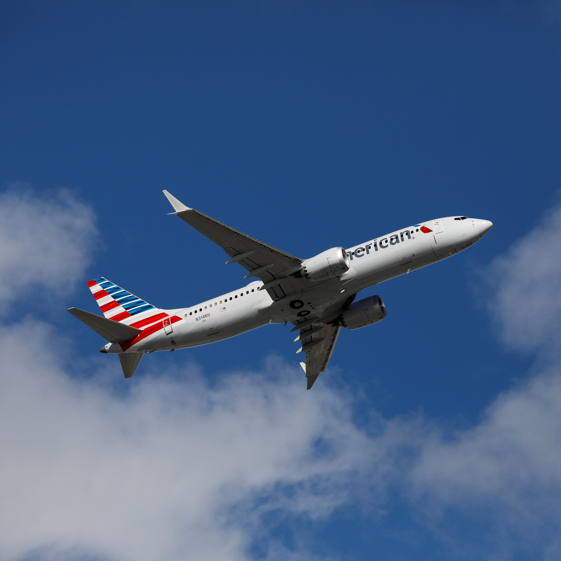Airplane	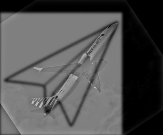sigma_low = 4 sigma_high = 10

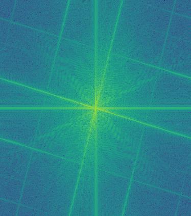
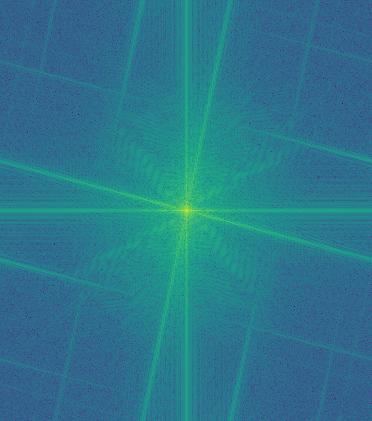
Fourier Analysis

I liked the way that comedy and tragedy turned out, so I performed Fourier analysis below.

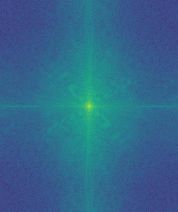Tragedy FFT	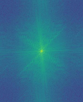Comedy FFT
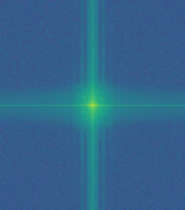Low Frequency FFT	High Frequency FFT

Hybrid Image FFT

Part 2.2 - Adding Color (Bells and Whistles)

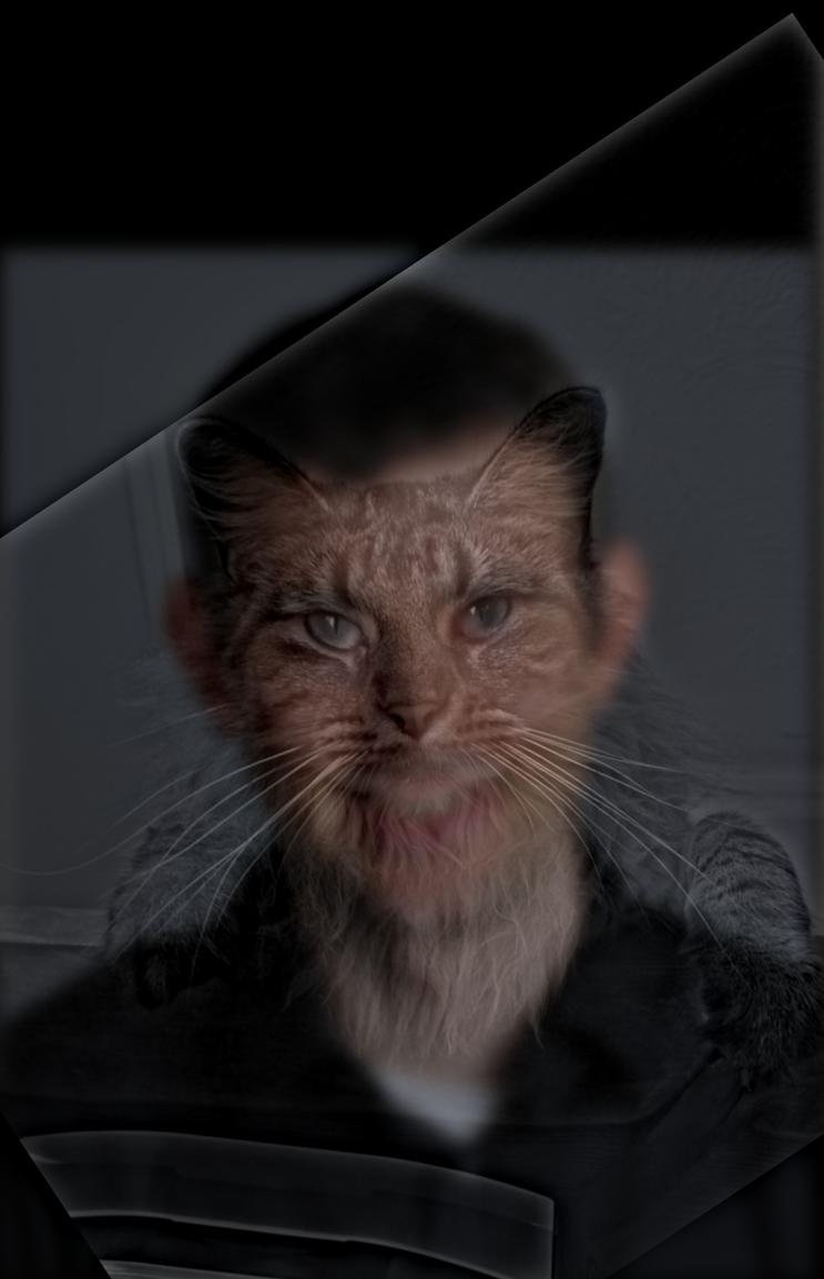
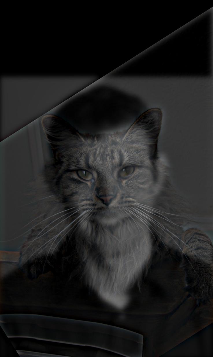
I experimented with using color on Derek and Nutmeg.

No Color	Low Frequency Color	High Frequency Color	Both Frequency Color

The color really only helps the low frequency image, considering that just using color on Nutmeg (high frequency) makes no difference. Using color on the low frequency image or both images makes it look different but not necessarily a lot better.

Part 2.3: Gaussian and Laplacian Stacks

We create Gaussian and Laplacian stacks for the input images. At every level of the Gaussian stack, we blur the previous image level with a kernel to get the current level’s image. We are using a Gaussian stack, which means that the image size remains the same. We can generate the Laplacian stack by using the Gaussian stack. At level i, l_stack[i] = g_stack[i] - g_stack[i+1]. At the last level i, l_stack[i] = g_stack[i]. This allows both stacks to have the same length. Each stack has 5 layers/levels.

Here are levels 0 through 4 of the input images’ Gaussian and Laplacian stacks. The Laplacian stack images here are normalized over the entire image (for visual purposes), but the un-normalized versions are using during computation.

Apple Gaussian Stack
Apple Laplacian Stack
Orange Gaussian Stack
Orange Laplacian Stack

Part 2.4: Multiresolution Blending

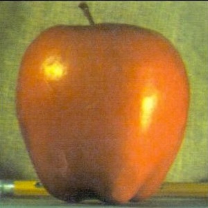
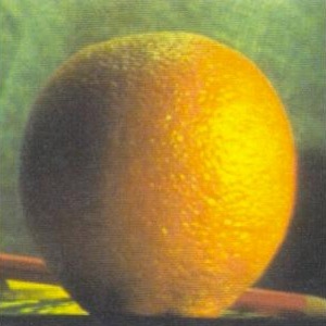
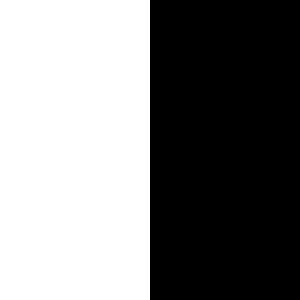
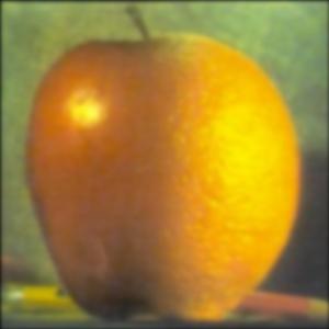
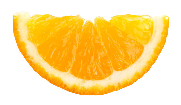
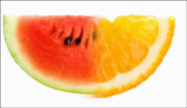
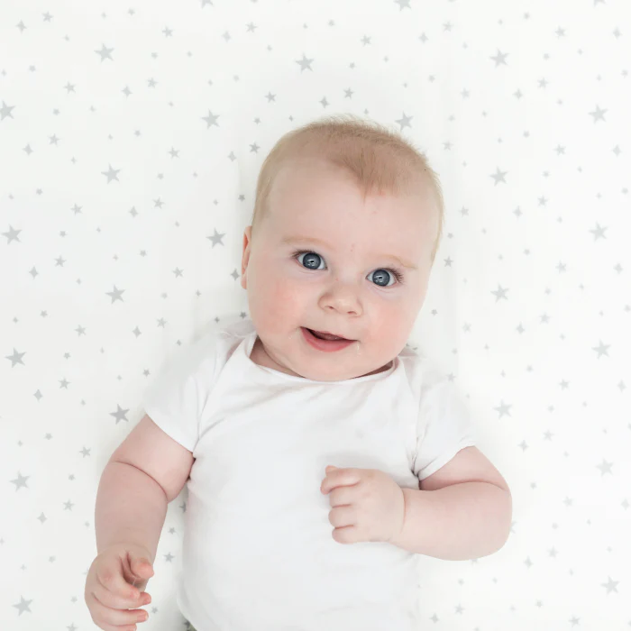
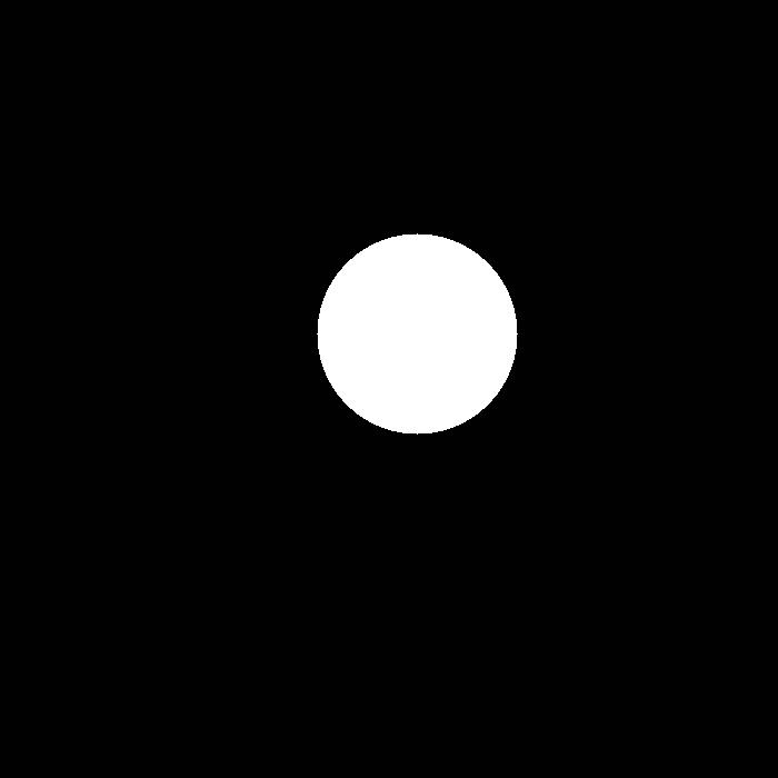
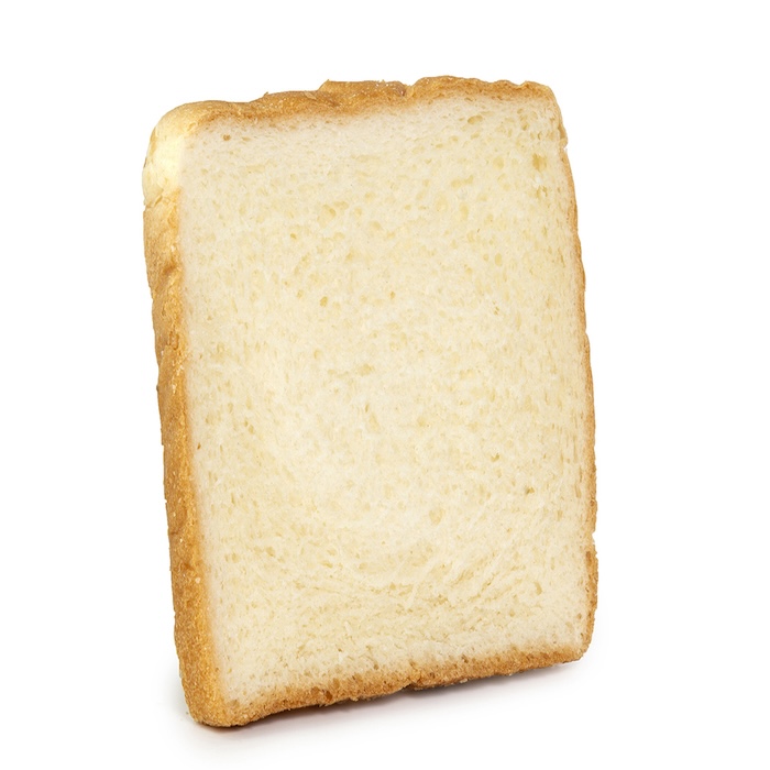
After I had the Gaussian and Laplacian stacks for the 2 input images as well as the Gaussian stack for the mask, I could blend everything together. I created the blended image by doing: blended_stack = g_stack_mask * l1_stack + (1 - g_stack_mask) * l2_stack. In addition to the oraple, I blended two other images (where the baby + bread blended image has an irregular mask). I used kernel_size = 12 and N = 5, with the exception of the Gaussian stack of the mask which had kernel_size = 60.

Image 1	Image 2	Mask	Blended Image
		Irregular Mask Example

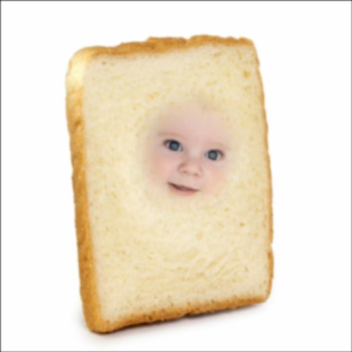Figure 3.42 Recreated

I created Figure 3.42 from the textbook on the oraple.

Level 0
Level 2
Level 4
Collapsed

Here is the final result again:

Image 1	Image 2	Blended Image

Conclusion

The most important thing I learned was how blended both the images and the mask using the Gaussian and Laplacian stacks helped the final image appear more realistic. As I refined my parameters, the output looked more smoothly blended and interesting to the viewer.